Category Archives: Tutorials

Polar alignment of the SkyWatcher Star Adventurer

The SkyWatcher Star Adventurer mount is a good quality equatorial tracking mount for DSLR based astrophotography. It is reasonably portable, so combined with a sturdy tripod, it is well suited for travel when weight & space are at a premium. It is not restricted to night time usage either, providing an option for tracking the movement of The Sun, making it suitable for general solar imaging / eclipse chasing too.

The key to getting good results from any tracking mount is to take care when doing the initial setup and alignment. The Star Adventurer comes with an illuminated polar scope to make this process easier. The simple way to use this is to rotate it so that the clock positions (3, 6, 9, 12) have their normal orientation, and then use a smart phone application to determine where Polaris should appear on the clock face. The alternative way is to use the date / time graduation circles to calculate the positioning from the date and time. Learning this process is helpful if your phone batteries die, or you simply want to avoid bright screens at night time.

The explanation of how to use the graduation circles in the manual is not as clear as it should be though, so this post attempts to walk through the process with some pictures along the way.

Observing location properties

The first thing to determine is the longitude & latitude of the observing location, by typing “coordinates <your town name>” into Google. In the case of Minneapolis it replies with

44.9778° N, 93.2650° W
The second piece of information required is the difference between the observing location longitude and the longitude associated with the timezone. Minnepolis is in the USA Central timezone which has a central meridian of 90° W, so the offset is:
93.2650° W - 90° W == 3.2650° W

Rough tripod alignment & mount assembly

Even though the Star Adventurer is a small portable mount, the combination of the mount, one or more cameras, and lens / short tube telescopes will have considerable weight. With this in mind, don’t try to get away with a light or compact tripod, use the strongest and heaviest tripod that you have available to support it well. When travelling, a trade off may have to be made to cope with luggage restrictions, which in turn can limit the length of exposures you can acquire and/or make it more susceptible to wind and vibrations. To increase the rigidity of any tripod, avoid fully extending the legs and keep them widely spaced. If the tripod has bracing between the legs use that, and if possible hang a heavy object beneath the tripod to damp any vibrations.

On this compact tripod the legs are only extended by 1/4 the normal length to maximize stability.

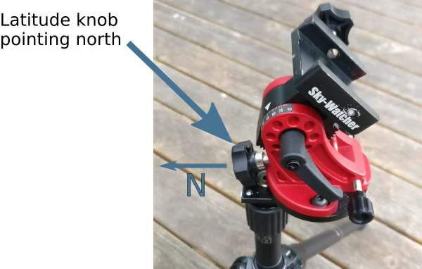
With the tripod erected, the first step is to attach the equatorial wedge. The tripod should be oriented so that the main latitude adjustment knob on the wedge is pointing approximately north. Either locate Polaris in the sky, or use a cheap hand held compass, or even a GPS app on a smart phone to determine north.

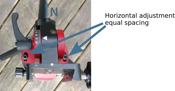
At this time also make sure that the two horizontal adjustment knobs are set to leave an equal amount of slack available in both directions. This will be needed when we come to fine tune the polar alignment later.

Now adjust the tripod legs to make the base of the wedge level, using the built-in omnidirectional spirit level to gauge it.

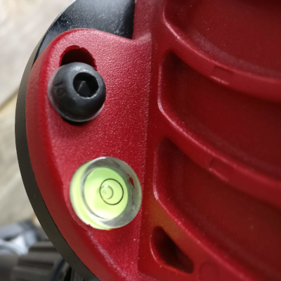
The spirit level on the wedge should have its bubble centred to ensure the tripod is level

The final part of the approximate alignment process is to use the altitude adjustment knob on the wedge to set the angle to match the current observing location latitude. As noted earlier the latitude of Minneapolis is 44.9778° N, so the altitude should be set to 45 too. Each major tick in the altitude scale covers 15°, and is subdivided into 5 minor ticks each covering .

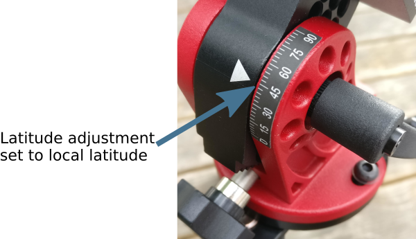
Latitude adjustment set to 45 corresponding to the latitude of Minneapolis

At this point the main axis of the mount should be pointing near to the celestial north pole, but this is not anywhere near good enough to avoid star trailing. The next step will to do the fine polar alignment.

Checking polar scope pattern calibration

For a mount that has not yet been used, it is advisable to check the calibration of the polar scope pattern, as it may not be correct upon delivery, especially if the unit has been used for demo purposes by the vendor or was a previous customer return. Once calibrated, it should stay correct for the lifetime of the product, so this won’t need repeating every time. Skip to the next heading if you know the pattern is correctly oriented already.

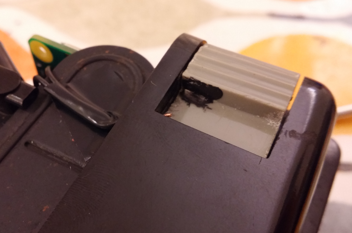
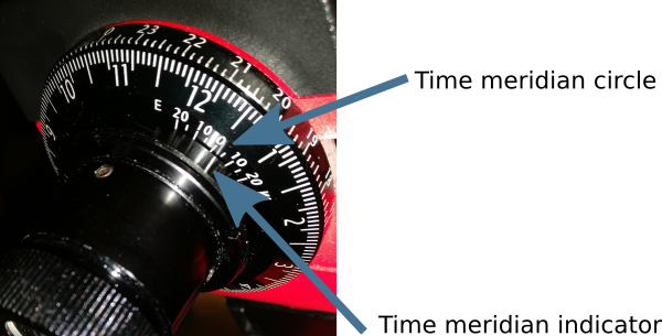
The rear of the main body has two graduated and numbered circles tracking time and date. The outer circle is fixed against the body and marked with numbers 0-23. Each of the large graduation marks represents 1 hour, while the small graduation marks represent 10 minutes each. The inner circle rotates freely and is marked with numbers 1 through 12. Each of the large graduation marks represents 1 month, while the small graduation marks represent approximately 2 days each. The inner circle has a second scale marked on it, with numbers 20, 10, 0, 10, 20 representing the time meridian offset in degrees. The eyepiece has a single white line painted on it which is the time meridian indicator.

To check calibration the inner circle needs to be rotated so that the time meridian circle zero position aligns with the time meridian indicator on the eyepiece.

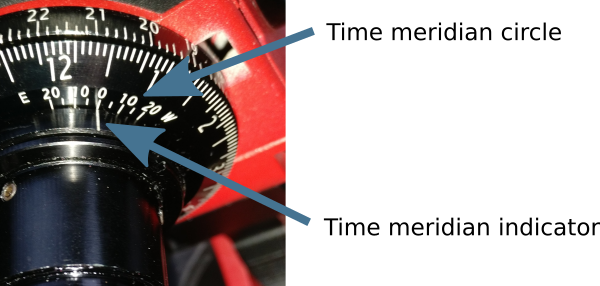
The zero position on the time meridian circle is aligned with the time meridian indicator mark on the eyepiece.

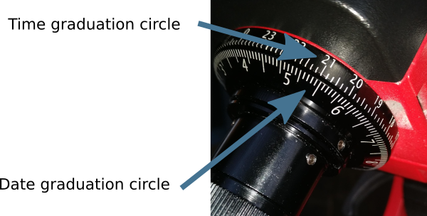
Now while being careful not to move the inner circle again, the mount axis / eyepiece needs to be rotated so that the zero mark on outer time graduation circle aligns with the date graduation circle Oct 31st mark (the big graduation between the 10 and 11 numbers).

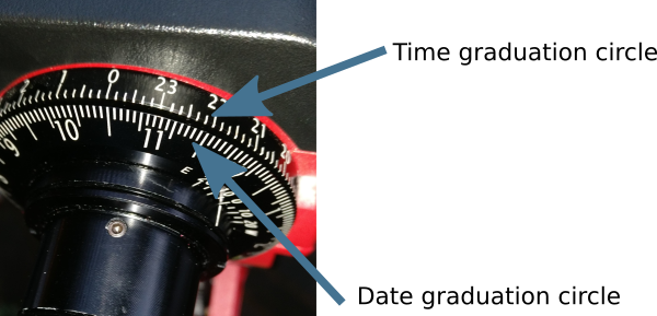
While not moving the inner cicle, the mount axis / eyepiece is rotated so that the number zero on the time graduation circle lines up with the large graduation between the 10 and 11 marks on the date graduation circle.

These two movements have set the mount to the date and time where Polaris will be due south of the north pole. Thus when looking through the eyepiece, the polar alignment pattern should appear with normal orientation, 6 at the bottom, 9 to the left, 3 to the right and 0 at the top. If this is not the case, then a tiny allen key needs to be used to loosen the screws holding the pattern, which can then be rotated to the correct orientation.

As mentioned above this process only needs to be done once when first acquiring the mount. Perhaps check it every 6-12 months, but it is very unlikely to have moved unless the screws holding the pattern were not tightened correctly.

Polar alignment procedure

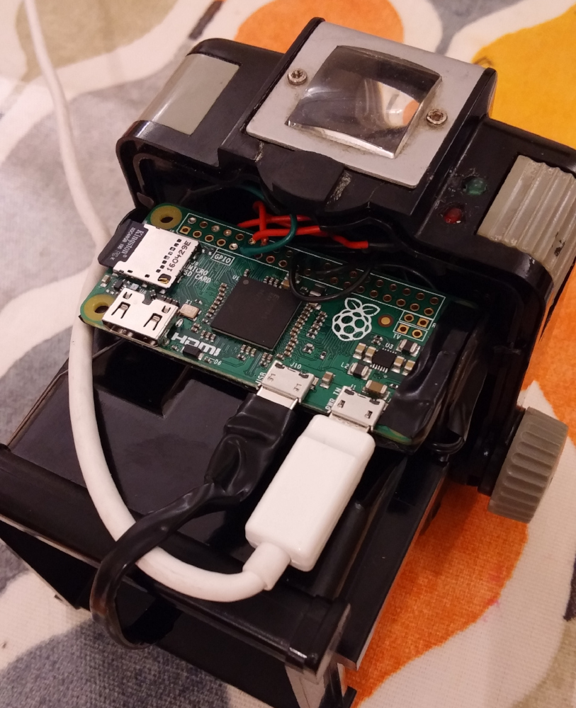
After getting the tripod setup with the wedge attached and main body mounted, the process of polar alignment can almost begin. First it is recommended to attach the mount assembly dovetail bar and any cameras to the mount body. It is possible to attach this after polar alignment, but there is the risk of movement on the mount which can ruin alignment. The only caveat with doing this is that with many versions of the mount it is impossible to attach the LED polar illuminator once the dovetail is attached. Current generations of the product ship an shim to solve this problem, while for older generations an equivalent adapter can be created with a 3-d printer and can often be found pre-printed on ebay.

Earlier the difference in longitude between the timezone meridian and the current observing location was determined to be 3.2650° W. The inner graduated disc on the mount needs to be rotated so that the time meridian indicator on the eyepiece points to the time meridian circle position corresponding to 3.2650° W

The time meridian indicator is aligned with the time meridian circle position corresponding to 3 W, which is the offset between the current observing location and the timezone meridian.

Now without moving the inner dial the main mount axis / eyepiece needs to be rotated to align the time graduation circle with the date graduation circle to match the current date and time. It is important to use the time without daylight saving applied. For example if observing on May 28th at 10pm, the time graduation circle marking for 21 needs to be used, not 22. May is the 5th month, and with each small graduation corresponding to 2 days, the date graduation circle needs to aligned for the graduation just before the big marker indicating June 1st.

The time graduation circle marking for 21 is aligned with the date graduation circle marking for May 28th.

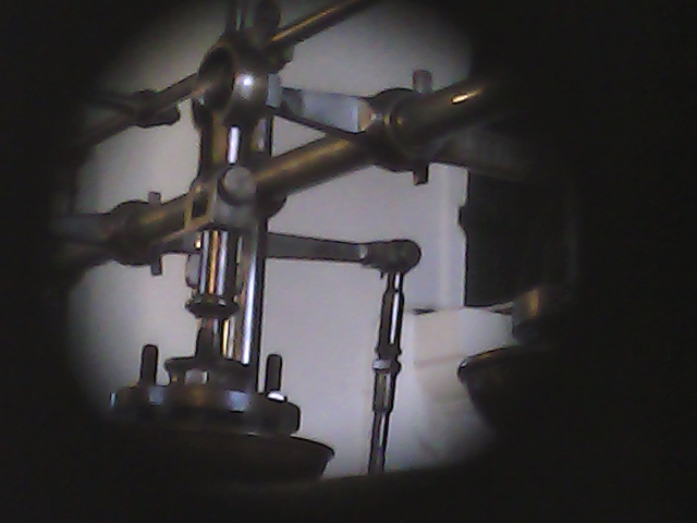
The effect of these two movements is to rotate the polar scope pattern so that the 6 o’clock position is pointing to where Polaris is supposed to lie. Hopefully Polaris is visible through the polar scope at this point, but it is very unlikely to be at the right position. The task is now to use the latitude adjustment knob and two horizontal adjustment knobs to fine tune the mount until Polaris is exactly at the 6 o’clock position on the pattern.

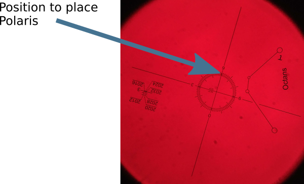
View of pattern through polar scope when set for 10pm on May 31st in Minneapolis, which is almost completely upside down. Polaris should be placed at the 6 o’clock position on the pattern.

Notice that the polar scope pattern has three concentric circles and off to the side of the pattern there are some year markings. Polaris gradually shifts from year to year, so check which of the concentric rings needs to be used for the current observing year.

The mount is now correctly aligned with the North celestial pole and should accurately track rotate of the Earth to allow exposures several minutes long without stars trailing. All that remains is to turn the power dial to activate tracking. One nice aspect of equatorial mounts compared to alt-az mounts, is that they can be turned off/on at will with no need to redo alignment. When adding or removing equipment, however, it is advisable to recheck the polar scope to ensure the mount hasn’t shifted its pointing.

The power dial set to normal speed tracking for stars.

Processing workflow for lunar surface images using GIMP and G’MIC

This post is going to illustrate a post-processing workflow for lunar surface images using the open source tools GIMP and G’MIC. GIMP has been largely ignored by astrophotographers in the past since it only supported 8-bit colour channels. The long awaited GIMP 2.10 release in April 2018, introduced 16-bit and 32-bit colour channel support, along with many other important improvements that enable high quality post-processing.

Astrophotographers seeking to present high detail images of The Moon, have long recognised that capturing a single still image is not sufficient. Instead normal practice is to capture a high definition video at a high frame rate lasting for a minute or more, by attaching a webcam to a telescope in place of the eyepiece. A program such as AutoStakkert2 will then process the video, analysing the quality of each video frame, selecting the “best” frames, and then merging them to produce a single frame with less noise and more detail. The output of AutoStakkert2 though is not a finished product and requires further post-processing to correct various image artefacts and pull out the inherent detail. A common tool used for this is Registax which particularly found popularity because of its wavelet sharpening feature.

Use of AutoStakkert2 can be a blog post in its own right, so won’t be covered here. What follows will pick up immediately after stacking has produced a merged image, and show how GIMP and G’MIC can replace use of the closed source, Windows based Registax tool.

The source material for the blog post is a 40 second long video captured with a modified Microsoft Lifecam HD paired with a Celestron Nexstar 4GT telescope. Most astrophotographers will spend £100 or more on CCD cameras directly designed for use with telescopes, so this modded Lifecam is very much at the low end of what can be used. This presents some extra challenges, but as can be seen, still allows for great results to be obtained with minimal expense.

The first noticeable characteristic of the video is a strong pink/purple colour cast on the edges of the frame. This is caused by unwanted infrared light reaching the webcam sensor. A IR cut filter is attached to the webcam, but it is positioned too far away from the CCD chip to be fully effective. A look at a single video frame at 100% magnification shows high level of speckled chromatic noise across the frame. Finally the image slowly drifts due to inaccurate tracking of The Moon’s movement by the telescope mount and features are stretched and squashed due to atmospheric distortion.

100% magnification crop of a single still video frame before any processing

After the video frames are stacked using AutoStakkert2, the resulting merged frame shows significant improvements. The speckled noise has been completely eliminated by the stacking process which effectively averages out the noise across 100s (even 1000s) of frames. The image, however, appears very soft lacking any fine detail and there is chromatic aberration present on the red and blue channels

100% magnification crop after stacking top (50% by quality) video frames in AutoStakkert2

AutoStakkert2 will save the merged image as a 16-bit PNG file, and GIMP 2.10 will honour this bit-depth when loading the image. It is possible to then convert it to 32-bit per channel before processing, but for lunar images this is probably overkill. The first task is to get rid of the chromatic aberration since that has the effect of making the image even softer. With this particular webcam and telescope combination it is apparent that the blue channel is shifted 2 or 3 pixels up, relative to the green, while the red is shifted 2 or 3 pixels down. It is possible to fix this in GIMP alone by decomposing the image, creating a layer for each colour channel, then moving the x,y offset of the blue and red layers until they line up with green, and finally recomposing the layers to a produce a new colour image.

This is a rather long winded process that is best automated, which is where G’MIC comes into play. It is a general purpose image processing tool which has the ability to run as a GIMP plugin, providing more than 450 image filters. The relevant filter for our purpose is called “Degradations -> Chromatic Aberrations“. It allows you to simply enter the desired x,y offset for the red and blue channels and will re-align them in one go, avoiding the multi-step decompose process in GIMP.

G’MIC Chromatic Aberration filter. The secondary colour defaults to green, but it is simpler if it is changed to blue, since that is the second fringe colour we’re looking to eliminate. The preview should be zoomed in to about 400% to allow alignment to be clearly viewed when adjusting x,y offsets.

100% magnification crop after aligning the RGB colour components to correct chromatic aberration.

With the chromatic aberration removed the next step is to get rid of the colour cast. The Moon is not a purely monochrome object, with different areas of its surface have distinct colours which would ideally be preserved in any processed images. Due to the limitations of the camera being used, however, the IR wavelength pollution makes that largely impossible/impractical. The only real option is to desaturate the image to create an uniformly monochrome image. If a slightly off-grey colour tint is desired in the end result, that could be added by colourizing the final image.

100% magnification crop after desaturating to remove colour cast due to IR wavelengths

The image that we have at this stage is still very soft, lacking in any fine detail. One of the most popular features in Registax is its wavelet based sharpening facility. Fortunately there are a number of options available in GIMP now that can achieve comparable results. GIMP 2.10 comes with a “Filters -> Enhance -> Wavelet decompose” operation, while G’MIC has “Details -> Split Details (wavelets)” both of which can get results comparable to Registax wavelets operating in linear mode. The preferred Registax approach though is to use guassian wavelets, and this has an equivalent in G’MIC available as “Details -> Split Details (gaussian)“. The way the G’MIC filter is used, however, is rather different so needs some explaining.

Split details (gaussian) filter. The image will be split into 6 layers by default, 5 layers of detail and a final background residual layer. Together the layers are identical to the original image. The number layers together with the two scale settings determine the granularity of detail in each layer. The defaults are reasonable but there’s scope to experiment if desired.

Describing the real mathematical principals behind gaussian wavelets is beyond the scope of this posting, but those interested can learn more from the AviStack implementation. Sticking to the high level, when the plugin is run it will split the visible layer into a sequence of layers. There is a base layer “residual” and then multiple layers of increasingly fine details applied with “Grain Merge” mode. Taken together these new layers are precisely equivalent to the original image.

The task now is to work on the individual detail layers to emphasize the details that are desired in the image, and (much less frequently) to de-emphasize details that are not desired. To increase the emphasis of details at a particular level, all that is required is to duplicate the appropriate layer. The finest detail layer may be duplicated many, many, many times while coarse detail layers may be duplicated only once, or not at all. If even one duplication is too strong, the duplicated layer opacity can be reduce to control its impact.

GIMP layers. The default G’MIC split details filter settings created 6 layers. The layer labelled “Scale #5” holds the fine details and has been duplicated 5 times to enhance fine details. The “Scale #4” and “Scale #3” layers have both been duplicated once, and opacity reduced on the “Scale #3” duplicate.

It is recommended to work in order from coarsest (“Scale #1”) to finest (“Scale #5”) detail layers, and typically the first two or three levels of details would be left unchanged to avoid unnatural looking images with too much contrast. There is no perfect set of wavelet adjustments that will provide the right amount of sharpening. It will vary depending on the camera, the telescope, the subject, the seeing conditions, the quality of stacking and more. Some experimentation will be required to find the right balance, but fortunately this is easy with layers since changes can be easily rolled back. After working on an image, ensure it is saved in GIMP’s native XCF format, leaving all layers intact. It that then be revisited the following day with a fresh eye whereupon the sharpening may be further fine tuned with benefit of hindsight.

100% magnification crop after sharpening using G’MIC gaussian wavelets filter and GIMP layer blending

As the image below shows, even with a modified webcam costing < £20 on a popular auction site, it is possible to produce high detail images of The Moon’s surface, using open source tools for all post-processing after the initial video stacking process.

Complete final image after all post-processing


Building a Kodak Brownie digital camera

The Kodak Brownie was the first camera to really bring photography to the masses with a low purchase price. The simplicity of its design meant anyone could figure out how to use it with little difficulty – even by comparison with today’s cameras it is still easy to use, since it has essentially no controls to learn – just a shutter button, view finder and film winder. Millions of Kodak Brownies were made over the course of its 60 year lifespan, from 1900 onwards and the build quality & simplicity means many survive in good working order. The upshot is that a Kodak Brownie is a good option for custom modifications – easily available on ebay or in car boot sales, simple to hack and cheap enough that it doesn’t matter if things go wrong.

The original plan was to build a variant on my previous raspberry pi & webcam based pinhole digital camera, since I already had a second raspberry pi zero needing a purpose. A previous trip to the local carboot sale had yielded a Kodak Brownie Hawkeye for less than £5, which is the variant from the 1950’s with a case made out of bakelite instead of wood / cardboard. So the only key missing piece was a webcam. Since both the raspberry pi zero and kodak brownie had cost less than £5, that was set as the upper limit for obtaining a webcam. Trawling eBay listings found a number of sellers offering a variety of 50 megapixel cameras at this price point. These technical specs were clearly complete & utter lies – it was never going to be a 50 MP sensor for that price – but at the same time it was worth a punt to discover just what the cameras did offer. I first one I obtained turned out to provide 640×480, or a mere 0.3 MP with raw video only, no mjpeg, thus limiting the framerate too. IOW pretty awful, but only marginally more awful than expected. The plus side was that the case was easy to remove exposing a very compact circuit board which would be an ideal size for embedding.

The “50 megapixel” eBay webcam, which turned out to be 0.3 megapixels, prior to removing the case

Upon testing the webcam with an improvised pinhole plate, it was clear that the sensor had unacceptably poor low-light performance. While it could serve as a pinhole camera, it would only be usable outside in bright conditions. I wanted to build a camera that was more versatile, so the plan was changed to build a “normal” digital camera instead of pinhole digital camera.

With the key parts obtained, design and assembly could begin. An initial approach was to keep the Brownie’s original lens and position the bare webcam sensor behind it. To achieve sharp focus, the sensor would have to be placed at the same position that the film would be relative to the lens. Each film negative, however, was 60x60mm in size, while the webcam sensor was less than 5x5mm. Testing confirmed that the webcam would have an incredibly narrow field of view, making it near impossible to compose shots with the crude viewfinder mirror.

The alternative was to disassemble the Brownie and remove its own plastic lens. The webcam circuit board could then be positioned such that its own lens was would be right behind the shutter. The circuit board was just a few mm to large to fit into the required position, so a dremmel tool was used to carve a slot in the inside of the case, allowing the circuit board to slip into place.

The interior of the Kodak Brownie, showing the circuit board in place immediately behind the lens. The circuit protrudes through a slot cut in the wall and held in place with bluetak.

This allowed the webcam to have a field of view similar to that of the original Brownie. In fact the field of view was wide enough that it covered the entire shutter aperture so the resulting images showed a circular vignette.

Still image captured by the webcam when behind the Kodak Brownie lens. The sensor field of view expands beyond the maximum size of the shutter aperture

The second task was deciding how to position to Raspberry Pi Zero in the case. As luck would have it, the width of the Pi Zero is exactly the same as the length of a 620 film spool, so the film holders were able to grip the Pi Zero circuit board. In common with the previous pinhole webcam, two LEDs were to be used, one illuminating when the power is on and one illuminating when the webcam is capturing an image. Two small holes were drilled in the top of the Brownie case next ot the shutter button, through which the LEDs could poke. A spot of superglue held the LEDs in the correct position.

Inside of Brownie case showing the Raspberry Pi Zero board, USB power cable and LED status indicators

One of the key goals for the camera design was that the shutter button on the Kodak Brownie should be used to trigger image capture on the webcam. Ideally a single press of the shutter button would capture a single image. To achieve this, the mechanical shutter button needed to interface with the Raspberry Pi GPIO pins in some manner. After thinking about this tricky problem for a while, a solution involving a pair of bare wires and some conductive paint was conceived. One wire would connect to a programmable GPIO pin configured as an input in pull-up mode. The second wire would connect to a GPIO ground pin. A hole was drilled through the case coming out immediately below the shutter button, through which the wires could pass. Insulation was stripped off the wires and they were superglued in position below the shutter button. Finally a blob of conductive paint was applied to the underside of the shutter button. The result is that when the shutter button is pressed, the conductive paint shorts out the two wires, pulling the GPIO pin to ground. This change can be detected by the Pi Zero and used to trigger the shutter.

Shutter button on the Kodak Brownie, showing a blob of conductive paint, used to short circuit wires used to trigger webcam capture

The Brownie shutter mechanism is designed for film with a fixed shutter speed. It was not practical to synchronize image capture with the precise fraction of a second that the shutter was open. Fortunately the Brownie has a long exposure mode where the shutter remains open for as long as the shutter button is pressed. Normally this long exposure mode is activated by raising a second button on the Brownie, but this is somewhat tedious. A little bit of electrical tape applied to the shutter mechanism was able to hook it into permanent long exposure mode.

The Brownie shutter mechanism with spot of electrical tape used to fix it in long exposure mode permanently.

Testing of the shutter mechanism was revealed a small problem – the webcam takes  a second or two to automatically measure & adjust exposure to suit the lighting conditions. The result was that if an image was captured immediately after pressing the shutter button, it would often be totally underexposed. This prompted another slight change in design. Rather than capturing a single image immediately as the shutter is pressed, the software was written to wait a second after shutter press and then capture images continuously thereafter, one per second, until the shutter was released. IOW, it would be a timelapse capture device.

The only remaining task was power. The Pi Zero and webcam combination has very low power requirements, at most 200 milliamps, and it was already known that a USB lithium ion powerpack provides an excellent power source that lasts a really long time. The problem is that for most powerpacks on sale today, physical size is not a hugely important factor. To date it has been impossible to find one that is small enough to fit inside the Brownie case – it would need to have a longest dimension of 6cm to stand a chance of fitting once the USB cable is plugged in – 5cm would be even better. Having the battery inside the case also adds a requirement to put a physical power switch between the Pi Zero and the battery, unless you want to open the camera to turn it on/off every time. The simple solution was thus to just drill a hole in the case for the USB cable, leaving the battery on the outside.

Finished Kodak Brownie digital camera showing cable to external battery pack

With the hardware construction complete, attention turned to the software to control it. Rather than start from scratch, the previous code used for the pinhole webcam Arcturus, was used extended. First it was discovered that the cheap webcam didn’t provide MJPEG capture, which meant pulling in libjpeg to do encoding of the raw frames into JPEG still image files. Capturing images in raw format means the USB device has to transfer far larger quantities of data. While this wasn’t a problem on the laptop used for development, the raspberry pi was continually getting dropped / incomplete frames from the webcam. After countless hours debugging, the problem was discovered to be the driver for the USB controller in Linux mainline, used by Pignus (the Fedora fork for the Raspberry Pi arm6 borads). The Raspbian kernel by comparison has an out of tree driver for the USB controller which turned out to work fine. The remaining software changes involved wiring up support for using the shutter button to trigger capture via a GPIO pin. The end result was that upon pressing the shutter button it would capture still images continuously, 1 per second. After a sufficiently long series of stills had been captured, they could be turned into a timelapse video sequence.